Input File: Basic Usage

In this documentation, we explain how to use block2 as an “executable”. The input parameters are provided in a formatted input file. The input file format used in block2 is highly compatible to the StackBlock format. For the most cases, the StackBlock input/configuration file (“dmrg.conf”) can be directly understood by block2, but block2 also has some important extension for the keywords.

The information provided below is analogous to the corresponding StackBlock documentation, since the same input file format is used. However, the output format of block2 can be very different from that of StackBlock.

Preparation

If block2 is installed using pip install block2, one can run a DMRG calculation using the following command:

block2main dmrg.conf > dmrg.out

Otherwise, for manual installation, please first compile the code according to Installation with cmake option -DBUILD_LIB=ON (and other necessary options). The following python script is used as the “block2 executable”:

${BLOCK2HOME}/pyblock2/driver/block2main

where ${BLOCK2HOME} is the block2 root directory. The build directory under block2 root directory should be in PYTHONPATH. You can add the following line in your environemnt (such as ~/.bashrc) or submission script:

export PYTHONPATH=${BLOCK2HOME}/build:${PYTHONPATH}

Then you can run a DMRG calculation using the following command:

${BLOCK2HOME}/pyblock2/driver/block2main dmrg.conf > dmrg.out

where dmrg.conf is the input file and dmrg.out is the output file.

To run a DMRG calculation with MPI parallelization, please use the following command:

mpirun --bind-to core --map-by ppr:${SLURM_TASKS_PER_NODE}:node:pe=${OMP_NUM_THREADS} \
    python -u ${BLOCK2HOME}/pyblock2/driver/block2main dmrg.conf > dmrg.out

where ${SLURM_TASKS_PER_NODE} is the number of mpi processes in each node. ${OMP_NUM_THREADS} is the number of threads (CPU cores) used by each mpi process. When executed in multiple nodes, a global scratch space (network file system) is required.

Integral Generation

In the following we will use the C₂ molecule to demonstrate the block2 features. Integrals and orbitals should be supplied externally in the Molpro’s FCIDUMP format. The integral file for C₂ can be found in ${BLOCK2HOME}/data/C2.CAS.PVDZ.FCIDUMP.ORIG or generated using the following script (only the RHF case is required):

from pyscf import gto, scf, mcscf
from pyblock2._pyscf.ao2mo import integrals as itg
from pyblock2.driver.core import DMRGDriver, SymmetryTypes

mol = gto.M(atom='C 0 0 0; C 0 0 1.2425', basis='ccpvdz', symmetry='d2h')

# RHF case (for spin-adapted / non-spin-adapted DMRG)
mf = scf.RHF(mol).run()
mc = mcscf.CASCI(mf, 26, 8)
ncas, n_elec, spin, ecore, h1e, g2e, orb_sym = itg.get_rhf_integrals(mf, mc.ncore, mc.ncas, g2e_symm=8)
driver = DMRGDriver(scratch="./tmp", symm_type=SymmetryTypes.SU2)
driver.initialize_system(n_sites=ncas, n_elec=n_elec, spin=spin, orb_sym=orb_sym)
driver.write_fcidump(h1e, g2e, ecore=ecore, filename='./FCIDUMP', pg="d2h", h1e_symm=True)

# UHF case (for non-spin-adapted DMRG only)
mf = scf.UHF(mol).run()
mc = mcscf.UCASCI(mf, 26, 8)
ncas, n_elec, spin, ecore, h1e, g2e, orb_sym = itg.get_uhf_integrals(mf, mc.ncore[0], mc.ncas, g2e_symm=8)
driver = DMRGDriver(scratch="./tmp", symm_type=SymmetryTypes.SZ)
driver.initialize_system(n_sites=ncas, n_elec=n_elec, spin=spin, orb_sym=orb_sym)
driver.write_fcidump(h1e, g2e, ecore=ecore, filename='./FCIDUMP.UHF', pg="d2h", h1e_symm=True)

Alternatively, the integral file can be generated using the pyscf/dmrgscf interface:

from pyscf import gto, scf, mcscf, dmrgscf
import os

dmrgscf.settings.BLOCKEXE = os.popen("which block2main").read().strip()
dmrgscf.settings.MPIPREFIX = ''

mol = gto.M(atom='C 0 0 0; C 0 0 1.2425', basis='ccpvdz', symmetry=1)
mf = scf.RHF(mol).run()
mc = mcscf.CASCI(mf, 26, 8)
mc.fcisolver = dmrgscf.DMRGCI(mol)
mc.canonicalization = False
dmrgscf.dryrun(mc)

Note

Please see DMRGSCF (pyscf) for the instruction for the installation of pyscf/dmrgscf.

Ground State Energy

The following input file can be used to compute the ground state energy:

sym d2h
orbitals C2.CAS.PVDZ.FCIDUMP.ORIG

nelec 8
spin 0
irrep 1

hf_occ integral
schedule default
maxM 500
maxiter 30
num_thrds 16

Note

Note that the integral file C2.CAS.PVDZ.FCIDUMP.ORIG should be in the working direcotry. By default, the orbitals will be reordered using the fiedler method. One can optionally add the keyword noreorder to avoid orbital reordering.

num_thrds indicates the number of OpenMP threads (shared-memory parallelism) to use.

hf_occ integral has no effects in block2, but it is required in StackBlock. If this line appears, block2main will try to write some output files in a stackblock-compatible format.

By default, the calculation will be done in the spin-adapted mode, which is the most efficient. One can optionally add the keyword nonspinadapted to use the non-spin-adapted mode.

The keyword prefix <scratch dir> can be used to set a folder for storing scratch files. If running in a HPC supercomputer, it is highly recommended to use the high IO speed scratch space (instead of the “home” storage) to achieve high performance.

Lines start with ! in the input file will be ignored. [1]

D_2h point group is enabled by sym d2h. The keywords schedule default and maxM sets the default sweep schedule and the maximum number of renormalized states kept during the sweep, respectively. block2 will then automatically set a sweep schedule as well as the defaults for various convergence thresholds.

The mps bond dimensions, sweep energies and the associated maximum discarded weights can be extracted by grepping the output dmrg.out.

$ grep Bond dmrg.out
Sweep =    0 | Direction =  forward | Bond dimension =  250 | Noise =  1.00e-03 | Dav threshold =  1.00e-04
Sweep =    1 | Direction = backward | Bond dimension =  250 | Noise =  1.00e-03 | Dav threshold =  1.00e-04
Sweep =    2 | Direction =  forward | Bond dimension =  250 | Noise =  1.00e-03 | Dav threshold =  1.00e-04
Sweep =    3 | Direction = backward | Bond dimension =  250 | Noise =  1.00e-03 | Dav threshold =  1.00e-04
... ...
Sweep =   16 | Direction =  forward | Bond dimension =  500 | Noise =  0.00e+00 | Dav threshold =  1.00e-06
Sweep =   17 | Direction = backward | Bond dimension =  500 | Noise =  0.00e+00 | Dav threshold =  1.00e-06
Sweep =    0 | Direction =  forward | Bond dimension =  500 | Noise =  0.00e+00 | Dav threshold =  1.00e-06
Sweep =    1 | Direction = backward | Bond dimension =  500 | Noise =  0.00e+00 | Dav threshold =  1.00e-06

$ grep DW dmrg.out
Time elapsed =      1.678 | E =     -75.4879935448 | DW = 1.39e-05
Time elapsed =      2.936 | E =     -75.6007921322 | DE = -1.13e-01 | DW = 9.88e-06
Time elapsed =      4.203 | E =     -75.6367659659 | DE = -3.60e-02 | DW = 9.25e-05
Time elapsed =      5.750 | E =     -75.6373954252 | DE = -6.29e-04 | DW = 3.91e-05
... ...
Time elapsed =     38.782 | E =     -75.7283521752 | DE = -3.48e-05 | DW = 5.24e-06
Time elapsed =     41.169 | E =     -75.7283676788 | DE = -1.55e-05 | DW = 5.28e-06
Time elapsed =      2.009 | E =     -75.7283421257 | DW = 4.18e-17
Time elapsed =      4.158 | E =     -75.7283421257 | DE = -2.84e-14 | DW = 2.47e-16

Note that in the last two sweeps (in default schedule) the 1-site algorithm is used. As a result, the discarded weights are nearly zero.

If you set outputlevel 1 in the input file, only essential information will be printed and the grep step can be skipped.

Targeting States

You can target the states distinguished by the number of electrons nelec, the total spin spin and the point-group symmetry of the state irrep.

The following input file computes the energy for a single B_1g state in D_2h point group:

sym d2h
orbitals C2.CAS.PVDZ.FCIDUMP.ORIG

nelec 8
spin 0
irrep 4

hf_occ integral
schedule default
maxM 500
maxiter 30

Note

In D_2h point group, irrep can be A_1g (1), B_3u (2), B_2u (3), B_1g (4), B_1u (5), B_2g (6), B_3g (7), A_1u (8).

This will generate the following output:

$ grep DW dmrg.out
Time elapsed =      1.983 | E =     -75.5422510106 | DW = 1.08e-05
Time elapsed =      3.580 | E =     -75.6245880097 | DE = -8.23e-02 | DW = 9.97e-06
Time elapsed =      5.376 | E =     -75.6366528654 | DE = -1.21e-02 | DW = 9.13e-05
Time elapsed =      7.172 | E =     -75.6374064699 | DE = -7.54e-04 | DW = 4.03e-05
... ...
Time elapsed =     38.611 | E =     -75.6389586629 | DE = -2.48e-05 | DW = 2.01e-06
Time elapsed =     40.981 | E =     -75.6389699555 | DE = -1.13e-05 | DW = 2.05e-06
Time elapsed =      2.029 | E =     -75.6389630224 | DW = 5.58e-15
Time elapsed =      4.106 | E =     -75.6389632670 | DE = -2.45e-07 | DW = 2.40e-16

State-Averaged Calculation

In the state-averaged DMRG algorithm, more than one state can be targeted in one calculation. The states being calculated can have the same or different nelec, spin or irrep. Multiple values can be given for the above keywords. [1] The number of states (roots) and the weight of each state can be specified using keywords nroots and weights, respectively. block2 will then try to find the low energy states within the space of targets formed by all combintaions of the given values of nelec, spin and irrep.

Note

In StackBlock, state-averaged calculation can only be done for states with the same nelec, spin and irrep. In block2, targetting multiple nelec, spin or irrep may cause the calculation hard to converge to the lowest energy states. Typically, one needs larger nroots than the number of states actually needed, to make sure that the low energy states are converged.

For normal non-state-averaged calculation, namely, when nroots is 1, you can also target multiple nelec, spin or irrep.

The following input file performs state-averged DMRG for two A_1g states in D_2h point group:

sym d2h
orbitals C2.CAS.PVDZ.FCIDUMP.ORIG

nelec 8
spin 0
irrep 1
nroots 2
weights 0.5 0.5

hf_occ integral
schedule default
maxM 500
maxiter 30

This will generate the following output:

$ grep DW dmrg.out
Time elapsed =      3.257 | E[  2] =     -75.5019604920    -75.4800275143 | DW = 1.54e-05
Time elapsed =      5.109 | E[  2] =     -75.5980474127    -75.5776457885 | DE = -9.76e-02 | DW = 1.98e-05
Time elapsed =      6.854 | E[  2] =     -75.6711500018    -75.6363593637 | DE = -5.87e-02 | DW = 1.86e-04
Time elapsed =      8.635 | E[  2] =     -75.6717525884    -75.6368970346 | DE = -5.38e-04 | DW = 1.35e-04
Time elapsed =     45.946 | E[  2] =     -75.7279558636    -75.6386525742 | DE = -3.41e-05 | DW = 2.49e-05
Time elapsed =     48.491 | E[  2] =     -75.7279954715    -75.6386699048 | DE = -1.73e-05 | DW = 1.67e-05
Time elapsed =      2.215 | E[  2] =     -75.7279403993    -75.6386251036 | DW = 1.77e-05
Time elapsed =      4.338 | E[  2] =     -75.7279224367    -75.6386152528 | DE = 9.85e-06 | DW = 8.35e-06

State-Specific Calculation

Orthogonalization Approach

The state-specific calculation can be done as a restart calculation which assumes that a previous state-averaged DMRG calculation has been converged. The state-specific DMRG calculation then reads the MPS from scratch folder and refines them for each root separately. The state-specific DMRG calculation can be done with any of onedot, twodot or twodot_to_onedot (default) keywords. [1]

Note

In StackBlock, state-specific calculation can only be done with onedot.

A state-specific DMRG calculation for two A_1g states in D_2h point group consists of two steps.

• First, using the input file given in the previous section to obtain the state-averaged MPSs (in the scratch folder).

• Second, the state-specific DMRG calculation can be performed by setting the keyword statespecific. The MPSs from the previous DMRG calculation will be read from the scratch folder. The following input file can be used for this step:

  sym d2h
  orbitals C2.CAS.PVDZ.FCIDUMP.ORIG
  
  nelec 8
  spin 0
  irrep 1
  nroots 2
  weights 0.5 0.5
  statespecific
  
  hf_occ integral
  schedule default
  maxM 500
  maxiter 30
  

This will generate the following output:

$ grep Energy dmrg.out
DMRG Energy for root    0 =  -75.728342642601376
DMRG Energy for root    1 =  -75.638959372610813

Sometimes, the orthogonalization approach can be unstable and when computing the exciated state it may fall back to the ground state. Adding the keyword onedot for the second step can alleviate this problem.

Level Shift Approach

The second step of the above can also be done with the level shift approach, by changing Hamiltonian from \(\hat{H}\) to \(\hat{H} + \sum_i w_i |\phi_i\rangle \langle \phi_i|\). Normally, the weights \(w_i\) are positive and they should be larger than the energy gap.

The following input file can be used for the second step:

sym d2h
orbitals C2.CAS.PVDZ.FCIDUMP.ORIG

nelec 8
spin 0
irrep 1
nroots 2
weights 0.5 0.5
statespecific
proj_weights 5 5

hf_occ integral
schedule default
maxM 500
maxiter 30

This will generate the following output:

$ grep Energy dmrg.out
DMRG Energy for root    0 =  -75.728341047222145
DMRG Energy for root    1 =  -75.638958637510370

Without State-Average

The excited MPS and energies can also be obtained without performing a state-averaged calculation as the first step. Instead, we can do several DMRG, and each time projecting out MPSs from all previous DMRG.

Note

It is recommended to use noreorder or fixed manual orbital reordering for this approach. Otherwise, one should carefully check that the orbital reordering in all DMRG calculations are the same.

We first get the ground state using the following input file dmrg-1.conf:

sym d2h
orbitals C2.CAS.PVDZ.FCIDUMP.ORIG

nelec 8
spin 0
irrep 1

schedule default
maxM 500
maxiter 30
mps_tags KET1

After this is finished, we compute the first excited state using the following input file dmrg-2.conf:

sym d2h
orbitals C2.CAS.PVDZ.FCIDUMP.ORIG

nelec 8
spin 0
irrep 1

schedule default
maxM 500
maxiter 30
mps_tags KET2

proj_mps_tags KET1
proj_weights 5

Then we compute the second excited state using the following input file dmrg-3.conf:

sym d2h
orbitals C2.CAS.PVDZ.FCIDUMP.ORIG

nelec 8
spin 0
irrep 1

schedule default
maxM 500
maxiter 30
mps_tags KET3

proj_mps_tags KET1 KET2
proj_weights 5 5

And so on.

This will generate the following output:

$ grep Energy dmrg-*.out
dmrg-1.out:DMRG Energy =  -75.728342508616663
dmrg-2.out:DMRG Energy =  -75.638961566176221
dmrg-3.out:DMRG Energy =  -75.629597871820607
dmrg-4.out:DMRG Energy =  -75.467766576734363
dmrg-5.out:DMRG Energy =  -75.350470798772307
dmrg-6.out:DMRG Energy =  -75.312672909521751

Mixed with State-Average

The above approach can also be used together with the state-average approach. Namely, we can first compute the two lowest states, then we compute the next three lowest states, by projecting out the two lowest states. The MPS to be projected must not be in state-averaged format, so we need to use the split_states keyword to break state-averaged MPS into individual MPSs, so that they can be used for projection in the subsequent calculations.

Currently, this type of state-average calulcation cannot be used together with multiple targets.

We first get the two lowest states using the following input file dmrg-1.conf:

sym d2h
orbitals C2.CAS.PVDZ.FCIDUMP.ORIG

nelec 8
spin 0
irrep 1
nroots 2
weights 0.5 0.5

schedule default
maxM 500
maxiter 30
mps_tags KET

copy_mps
split_states

After this is finished, we compute the next three states using the following input file dmrg-2.conf:

sym d2h
orbitals C2.CAS.PVDZ.FCIDUMP.ORIG

nelec 8
spin 0
irrep 1
nroots 3
weights 0.5 0.5 0.5

schedule default
maxM 500
maxiter 30
mps_tags EXKET

proj_mps_tags KET-0 KET-1
proj_weights 5 5

copy_mps
split_states

After this is finished, we compute the next one state using the following input file dmrg-3.conf:

sym d2h
orbitals C2.CAS.PVDZ.FCIDUMP.ORIG

nelec 8
spin 0
irrep 1

schedule default
maxM 500
maxiter 30
mps_tags EXXKET

proj_mps_tags KET-0 KET-1 EXKET-0 EXKET-1 EXKET-2
proj_weights 5 5 5 5 5

This will generate the following output:

$ grep DW dmrg-1.out | tail -1
Time elapsed =      5.461 | E[  2] =     -75.7279224622    -75.6386156808 | DE = 9.32e-06 | DW = 8.33e-06
$ grep DW dmrg-2.out | tail -1
Time elapsed =     13.165 | E[  3] =     -75.6290377907    -75.4669665917    -75.3494878435 | DE = 8.63e-07 | DW = 8.45e-05
$ grep DW dmrg-3.out | tail -1
Time elapsed =      8.651 | E =     -75.3126745298 | DE = -6.24e-07 | DW = 3.79e-15

n-Particle Reduced Density Matrix

The 1-, 2-, 3-, and 4-particle DMRG reduced density matrix for a particular state can be calculated using the keywords onepdm, twopdm, threepdm and fourpdm. The reduced density matrix calculation can be done with either onedot or twodot keywords. [1]

Note

Most of the time, only onedot density matrix calculation makes sense, since the MPS should not change during the sweep.

Density matrices of the \(n\)-th state are calculated and stored in a numpy binary file named 1pdm-n-n.npy, 2pdm-n-n.npy, 3pdm-n-n.npy, etc. (in the scratch folder), respectively, starting with n = 0. If there is only one root, the files are named 1pdm.npy, 2pdm.npy, 3pdm.npy, etc. respectively.

The following input file computes the energy and 2-particle density matrix for the ground state:

sym d2h
orbitals C2.CAS.PVDZ.FCIDUMP.ORIG

nelec 8
spin 0
irrep 1

schedule default
maxM 500
maxiter 30

twopdm
num_thrds 16

The 2-particle density matrix file can be loaded using the following python script:

>>> import numpy as np
>>> _2pdm = np.load('./nodex/2pdm.npy')
>>> print(_2pdm.shape)
(3, 26, 26, 26, 26)

The following input file computes the energy and 2-particle density matrix for two state-averaged A_1g states:

sym d2h
orbitals C2.CAS.PVDZ.FCIDUMP.ORIG

nelec 8
spin 0
irrep 1
nroots 2
weights 0.5 0.5

schedule default
maxM 500
maxiter 30

twopdm
num_thrds 16

The 2-particle density matrix file for the first state can be loaded using the following python script:

>>> import numpy as np
>>> n = 0
>>> _2pdm = np.load('./nodex/2pdm-%d-%d.npy' % (n, n))
>>> print(_2pdm.shape)
(3, 26, 26, 26, 26)

The 1-particle density matrix (in both the non-spin-adapted and spin-adapted mode) is stored as an array with the shape \([2,n,n]\), where n is the number of spatial orbitals, and the two components with indicies \([:,a,b]\) are for \(\langle a^\dagger_{a\alpha} a_{b\alpha} \rangle\), and \(\langle a^\dagger_{a\beta} a_{b\beta} \rangle\), respectively.

The 2-particle density matrix (in both the non-spin-adapted and spin-adapted mode) is stored as an array with the shape \([3,n,n,n,n]\), where the three components with indicies \([:,a,b,c,d]\) are for \(\langle a^\dagger_{a\alpha} a^\dagger_{b\alpha} a_{c\alpha} a_{d\alpha} \rangle\), \(\langle a^\dagger_{a\alpha} a^\dagger_{b\beta} a_{c\beta} a_{d\alpha} \rangle\), and \(\langle a^\dagger_{a\beta} a^\dagger_{b\beta} a_{c\beta} a_{d\beta} \rangle\), respectively.

The 3-particle density matrix in the spin-adapted mode is stored as the spin-traced format with the shape \([n,n,n,n,n,n]\), defined as

\[\text{3pdm}[a, b, c, d, e, f] := \sum_{\sigma\tau\lambda} a^\dagger_{a\sigma} a^\dagger_{b\tau} a^\dagger_{c\lambda} a_{d\lambda} a_{e\tau} a_{f\sigma}\]

The 3-particle density matrix in the non-spin-adapted mode is stored as an array with the shape \([4,n,n,n,n,n,n]\), where the four components with indicies \([:,a,b,c,d,e,f]\) are for \(\langle a^\dagger_{a\alpha} a^\dagger_{b\alpha} a^\dagger_{c\alpha} a_{d\alpha}a_{e\alpha} a_{f\alpha} \rangle\), \(\langle a^\dagger_{a\alpha} a^\dagger_{b\alpha} a^\dagger_{c\beta} a_{d\beta}a_{e\alpha} a_{f\alpha} \rangle\), \(\langle a^\dagger_{a\alpha} a^\dagger_{b\beta} a^\dagger_{c\beta} a_{d\beta}a_{e\beta} a_{f\alpha} \rangle\), and \(\langle a^\dagger_{a\beta} a^\dagger_{b\beta} a^\dagger_{c\beta} a_{d\beta}a_{e\beta} a_{f\beta} \rangle\), respectively.

The 4-particle density matrix in the spin-adapted mode is stored as the spin-traced format with the shape \([n,n,n,n,n,n,n,n]\), defined as

\[\text{4pdm}[a, b, c, d, e, f, g, h] := \sum_{\sigma\tau\lambda\mu} a^\dagger_{a\sigma} a^\dagger_{b\tau} a^\dagger_{c\lambda} a^\dagger_{d\mu} a_{e\mu}a_{f\lambda} a_{g\tau} a_{h\sigma}\]

The 4-particle density matrix in the non-spin-adapted mode is stored as an array with the shape \([5,n,n,n,n,n,n,n,n]\), where the five components with indicies \([:,a,b,c,d,e,f,g,h]\) are for \(\langle a^\dagger_{a\alpha} a^\dagger_{b\alpha} a^\dagger_{c\alpha} a^\dagger_{d\alpha} a_{e\alpha} a_{f\alpha} a_{g\alpha} a_{h\alpha} \rangle\), \(\langle a^\dagger_{a\alpha} a^\dagger_{b\alpha} a^\dagger_{c\alpha} a^\dagger_{d\beta} a_{e\beta} a_{f\alpha} a_{g\alpha} a_{h\alpha} \rangle\), \(\langle a^\dagger_{a\alpha} a^\dagger_{b\alpha} a^\dagger_{c\beta} a^\dagger_{d\beta} a_{e\beta} a_{f\beta} a_{g\alpha} a_{h\alpha} \rangle\), \(\langle a^\dagger_{a\alpha} a^\dagger_{b\beta} a^\dagger_{c\beta} a^\dagger_{d\beta} a_{e\beta} a_{f\beta} a_{g\beta} a_{h\alpha} \rangle\), and \(\langle a^\dagger_{a\beta} a^\dagger_{b\beta} a^\dagger_{c\beta} a^\dagger_{d\beta} a_{e\beta} a_{f\beta} a_{g\beta} a_{h\beta} \rangle\), respectively.

In the general spin orbital mode (with the keyword use_general_spin), the 1-, 2-, 3-, and 4-particle density matrices are stored with the shape \([1,n,n]\), \([1,n,n,n,n]\), \([1,n,n,n,n,n,n]\), and \([1,n,n,n,n,n,n,n,n]\) respectively, where n is the number of spin orbitals. The content is the expectation value for \(\langle a^\dagger_{a} a_{b} \rangle\), \(\langle a^\dagger_{a} a^\dagger_{b} a_{c} a_{d} \rangle\), \(\langle a^\dagger_{a} a^\dagger_{b} a^\dagger_{c} a_{d} a_{e} a_{f} \rangle\), and \(\langle a^\dagger_{a} a^\dagger_{b} a^\dagger_{c} a^\dagger_{d} a_{e} a_{f} a_{g} a_{h} \rangle\), respectively.

n-Particle Transition Reduced Density Matrix

The 1-, 2-, 3- and 4-particle DMRG transition density matrix can be calculated using the keywords tran_onepdm, tran_twopdm, tran_threepdm and tran_fourpdm.

Transition density matrices between the \(m\)-th (bra) and \(n\)-th (ket) states are calculated and stored in a numpy binary file named 1pdm-m-n.npy, 2pdm-m-n.npy, etc. (in the scratch folder), respectively, starting with m = n = 0.

The following input file computes the 2-particle transition density matrix for two state-averaged A_1g states:

sym d2h
orbitals C2.CAS.PVDZ.FCIDUMP.ORIG

nelec 8
spin 0
irrep 1
nroots 2
weights 0.5 0.5

schedule default
maxM 500
maxiter 30

tran_twopdm
num_thrds 16

Note

There can be a overall undetermined +1/-1 factor in Transition density matrices due to the relative phase in two MPSs.

The following input file computes the state-specific 2-particle transition density matrix for two refined A_1g states:

sym d2h
orbitals C2.CAS.PVDZ.FCIDUMP.ORIG

nelec 8
spin 0
irrep 1
nroots 2
weights 0.5 0.5
statespecific

schedule default
maxM 500
maxiter 30

tran_twopdm
num_thrds 16

The transition density matrices between states with different point group irreducible representations are also available by simply adding the keyword tran_twopdm after the corresponding multi-target state-averaged calculation. [1]

Restart DMRG Energy Calculation

DMRG energy calculations can be restarted, using the MPS (stored in scratch folder) generated in the previous calculation, by specifying the keyword fullrestart. If the previous calulcation stopped during the middle of a sweep, it will be restarted from the middle of a sweep.

Alternatively, the user can also set a directory for storing MPS after each sweep using the keyword restart_dir. [1] When restarting, the MPS data and mps_info.bin in the scratch folder should be copied from the restart_dir to the scartch folder of the restarting calculation.

The keyword restart_dir_per_sweep can be used to save a copy of MPS for each sweep. The MPS from different sweeps will be put into different folders (by adding suffix to the given direcotry).

You may need to change the (custom) scheudle in the input file so that the sweeps (with smaller bond dimension) finished in previous calculations will not be repeated, when you are restarting an interrupted calculation.

The following input file restarts an interrupted calculation:

sym d2h
orbitals C2.CAS.PVDZ.FCIDUMP.ORIG

nelec 8
spin 0
irrep 1

hf_occ integral
schedule default
maxM 500
maxiter 30

fullrestart

Load MPS for Density Matrix Calculation

The density matrix and transition density matrix calculation can be carried out separately, by restarting from an existing MPS, state-averged MPSs or state-specific MPSs (stored in scartch folder from a previous DMRG energy calculation).

Assuming a previous ground-state energy calculation has been finished, the following input file computes the 2-particle density matrix for the ground-state (loaded from scratch folder):

sym d2h
orbitals C2.CAS.PVDZ.FCIDUMP.ORIG

nelec 8
spin 0
irrep 1

hf_occ integral
schedule default
maxM 500
maxiter 30

restart_twopdm

Assuming a previous state-averaged energy calculation has been finished, the following input file computes the 2-particle transition density matrix for two state-averaged A_1g states (loaded from scratch folder):

sym d2h
orbitals C2.CAS.PVDZ.FCIDUMP.ORIG

nelec 8
spin 0
irrep 1
nroots 2
weights 0.5 0.5

hf_occ integral
schedule default
maxM 500
maxiter 30

restart_tran_twopdm

Now we explain how to compute 2-particle transition density matrix for bra and ket states belonging to different point group irreducible representations. We consider the A_1g (bra) and B_3u (ket) states.

The following input file computes the energy for a single B_3u state in D_2h point group. The keyword mps_tags can be used to assign a tag to the mps for later reference: [1]

sym d2h
orbitals C2.CAS.PVDZ.FCIDUMP.ORIG

nelec 8
spin 0
irrep 2

hf_occ integral
schedule default
maxM 500
maxiter 30

mps_tags KET
num_thrds 16

The following input file computes the energy for a single A_1g state in D_2h point group:

sym d2h
orbitals C2.CAS.PVDZ.FCIDUMP.ORIG

nelec 8
spin 0
irrep 1

hf_occ integral
schedule default
maxM 500
maxiter 30

mps_tags BRA
num_thrds 16

The output looks like the following:

$ grep Energy dmrg-1.out
DMRG Energy =  -75.675393353797631
$ grep Energy dmrg-2.out
DMRG Energy =  -75.728342388135175

The following input file computes the 2-particle transition density matrix for the two states:

sym d2h
orbitals C2.CAS.PVDZ.FCIDUMP.ORIG

nelec 8
spin 0
irrep 1
mps_tags BRA KET

hf_occ integral
schedule default
maxM 500
maxiter 30
restart_tran_twopdm
num_thrds 16

Note that in the above input file, keywords such as nelec, spin, irrep, and nroots will be unimportant. The keyword mps_tags lists the tags for the MPSs that should be loaded. [1]

Diagonal 2-Particle Density Matrix

Since the full two-particle density matrix calculation can be expensive for some systems, it is possible to calculate only the diagonal parts, which is much cheaper, using the keywords restart_diag_twopdm or diag_twopdm. [1] The time cost for diagonal 2pdm is roughly 2 times of the cost of 1pdm.

Note that diag_twopdm implies onepdm and correlation. The diagonal 2pdm is defined as:

\[\begin{split}e_{pqqp} \equiv&\ \sum_{\sigma\tau} \langle a_{p\sigma}^\dagger a_{q\tau}^\dagger a_{q\tau} a_{p\sigma} \rangle = -\sum_{\sigma\tau} \langle a_{p\sigma}^\dagger a_{q\tau}^\dagger a_{p\sigma} a_{q\tau} \rangle = \sum_{\sigma\tau} \langle a_{p\sigma}^\dagger a_{p\sigma} a_{q\tau}^\dagger a_{q\tau} \rangle - \delta_{pq} \sum_{\sigma} \langle a_{p\sigma}^\dagger a_{q\sigma} \rangle \\ =&\ \sum_{\sigma\tau} \langle n_{p\sigma} n_{q\tau} \rangle - \delta_{pq} \sum_{\sigma} \langle a_{p\sigma}^\dagger a_{q\sigma} \rangle \\ e_{pqpq} \equiv&\ \sum_{\sigma\tau} \langle a_{p\sigma}^\dagger a_{q\tau}^\dagger a_{p\tau} a_{q\sigma} \rangle = -\sum_{\sigma\tau} \langle a_{p\sigma}^\dagger a_{p\tau} a_{q\tau}^\dagger a_{q\sigma} \rangle + \delta_{pq} \sum_{\sigma\tau} \langle a_{p\sigma}^\dagger a_{q\sigma} \rangle \\ =&\ -\sum_{\sigma\tau} \langle a_{p\sigma}^\dagger a_{p\tau} a_{q\tau}^\dagger a_{q\sigma} \rangle + 2\delta_{pq} \sum_{\sigma} \langle a_{p\sigma}^\dagger a_{q\sigma} \rangle\end{split}\]

The computed diagonal 2pdm will be stored as e_pqqp.npy and e_pqpq.npy in scratch folder.

If one also computed the full 2pdm using the keyword twopdm or restart_twopdm, we can verify that its diagonal part matches the e_pqqp.npy and e_pqpq.npy obtained here:

>>> import numpy as np
>>> _2pdm = np.load('./nodex/2pdm.npy')
>>> print(_2pdm.shape)
(3, 26, 26, 26, 26)
>>> _e_pqqp = np.load('./nodex/e_pqqp.npy')
>>> _e_pqpq = np.load('./nodex/e_pqpq.npy')
>>> _2pdm_spat = _2pdm[0] + 2 * _2pdm[1] + _2pdm[2]
>>> _2pdm_spat_pqqp = np.einsum('pqqp->pq', _2pdm_spat)
>>> _2pdm_spat_pqpq = np.einsum('pqpq->pq', _2pdm_spat)
>>> print(np.linalg.norm(_e_pqqp - _2pdm_spat_pqqp))
3.28666776770176e-14
>>> print(np.linalg.norm(_e_pqpq - _2pdm_spat_pqpq))
1.6947732597975102e-14

Custom Sweep Schedule

The sweep schedule defines number of the renormalized states \(M\) kept , the convergence threshold for Davidson algorithm (in the unit of norm²), and the noise (in the unit of norm²) in successive DMRG sweeps. For finer control over the sweeps, customized sweep schedule should be used.

The following input file computes the ground state energy using a custom sweep schedule:

sym d2h
orbitals C2.CAS.PVDZ.FCIDUMP.ORIG

nelec 8
spin 0
irrep 1

hf_occ integral
schedule
0  100  1E-4  1E-3
4  250  1E-4  1E-3
8  400  1E-5  1E-4
10 600  1E-6  1E-5
12 800  1E-7  1E-6
14 1000 1E-8  1E-7
16 1000 1E-8  0E+0
end
twodot_to_onedot 18
maxiter 100
sweep_tol 1E-9

In the above input file, twodot_to_onedot specifies the sweep at which the switch is made from a 2-site to a 1-site DMRG algorithm (counting from 0). maxiter gives the maximum number of sweep iterations to be performed. sweep_tol gives the final tolerance on the DMRG energy, and is analogous to an energy convergence threshold in other quantum chemistry methods.

In the above input file, between schedule and end each line has four values. They are corresponding to starting sweep iteration (counting from zero), MPS bond dimension, tolerance for the Davidson iteration, and noise, respectively. Starting sweep iteration is the sweep iteration in which the given parameters in the line should take effect.

This will generate the following output:

$ grep DW dmrg.out
Time elapsed =      1.686 | E =     -74.1599100997 | DW = 4.86e-05
Time elapsed =      3.332 | E =     -74.6555553068 | DE = -4.96e-01 | DW = 7.28e-05
Time elapsed =      4.461 | E =     -75.6224601188 | DE = -9.67e-01 | DW = 1.55e-04
Time elapsed =      5.648 | E =     -75.6302268887 | DE = -7.77e-03 | DW = 1.26e-04
Time elapsed =      7.491 | E =     -75.6347292246 | DE = -4.50e-03 | DW = 6.46e-05
Time elapsed =     10.732 | E =     -75.6367873793 | DE = -2.06e-03 | DW = 2.96e-05
Time elapsed =     13.383 | E =     -75.6372588510 | DE = -4.71e-04 | DW = 1.01e-04
Time elapsed =     16.138 | E =     -75.6375874124 | DE = -3.29e-04 | DW = 3.83e-05
Time elapsed =     20.541 | E =     -75.6687725683 | DE = -3.12e-02 | DW = 8.76e-06
Time elapsed =     26.404 | E =     -75.7265879915 | DE = -5.78e-02 | DW = 9.21e-06
Time elapsed =     36.001 | E =     -75.7282887562 | DE = -1.70e-03 | DW = 3.43e-06
Time elapsed =     47.351 | E =     -75.7283943399 | DE = -1.06e-04 | DW = 3.04e-06
Time elapsed =     64.673 | E =     -75.7284858001 | DE = -9.15e-05 | DW = 1.24e-06
Time elapsed =     86.412 | E =     -75.7285031554 | DE = -1.74e-05 | DW = 1.21e-06
Time elapsed =    118.443 | E =     -75.7285302492 | DE = -2.71e-05 | DW = 4.82e-07
Time elapsed =    158.894 | E =     -75.7285335786 | DE = -3.33e-06 | DW = 5.44e-07
Time elapsed =    176.071 | E =     -75.7285376489 | DE = -4.07e-06 | DW = 5.73e-07
Time elapsed =    191.672 | E =     -75.7285377336 | DE = -8.46e-08 | DW = 5.76e-07
Time elapsed =     10.790 | E =     -75.7285342605 | DW = 1.47e-16
Time elapsed =     21.186 | E =     -75.7285342992 | DE = -3.87e-08 | DW = 3.21e-14
Time elapsed =     31.924 | E =     -75.7285343224 | DE = -2.32e-08 | DW = 3.07e-17
Time elapsed =     42.348 | E =     -75.7285343375 | DE = -1.51e-08 | DW = 8.17e-15
Time elapsed =     53.073 | E =     -75.7285343475 | DE = -9.98e-09 | DW = 4.35e-17
Time elapsed =     63.362 | E =     -75.7285343571 | DE = -9.58e-09 | DW = 6.64e-16
Time elapsed =     73.965 | E =     -75.7285343630 | DE = -5.87e-09 | DW = 3.96e-17
Time elapsed =     84.094 | E =     -75.7285343661 | DE = -3.17e-09 | DW = 1.14e-16
Time elapsed =     94.525 | E =     -75.7285343678 | DE = -1.71e-09 | DW = 1.34e-16
Time elapsed =    104.658 | E =     -75.7285343721 | DE = -4.29e-09 | DW = 2.45e-16
Time elapsed =    114.925 | E =     -75.7285343746 | DE = -2.44e-09 | DW = 1.38e-16
Time elapsed =    124.710 | E =     -75.7285343763 | DE = -1.76e-09 | DW = 3.03e-16
Time elapsed =    135.115 | E =     -75.7285343763 | DE = 5.68e-14 | DW = 2.24e-17

Sweep Energy Extrapolation

In practice the sweep energy converges almost linearly as a function of the “maximum discarded weight”. Therefore, it is convenient to use the “maximum discarded weight” quantity as an estimate of the error of the DMRG calculation. It is recommended to use the 2-site algorithm for energy extrapolation since the 2-site DMRG wavefunction provides additional variational freedom over the 1-site DMRG wavefunction. A strong deviation from a linear function (e.g. a plateau behavior followed by a sudden drop of the energy as a function of discarded weight) indicates that the DMRG was stuck in a local minimum.

One can use restart a converged DMRG calculation with a “reverse schedule” to generate data for energy extrapolation. This can guarentee that the energy for each different MPS bond dimension is fully converged and not representing any local minima.

The following input file restarts the previous calculation using a custom reverse sweep schedule:

sym d2h
orbitals C2.CAS.PVDZ.FCIDUMP.ORIG

nelec 8
spin 0
irrep 1

hf_occ integral
twodot
schedule
0  800  1E-8  0E+0
4  600  1E-8  0E+0
8  400  1E-8  0E+0
12 200  1E-8  0E+0
end
maxiter 16
sweep_tol 0.0
fullrestart

This will generate the following output (dmrg-2.out):

$ grep DW dmrg-2.out
Time elapsed =     12.597 | E =     -75.7285358881 | DW = 1.75e-06
Time elapsed =     23.720 | E =     -75.7285188420 | DE = 1.70e-05 | DW = 1.42e-06
Time elapsed =     33.955 | E =     -75.7285186195 | DE = 2.23e-07 | DW = 1.35e-06
Time elapsed =     44.842 | E =     -75.7285186529 | DE = -3.34e-08 | DW = 1.34e-06
Time elapsed =     52.432 | E =     -75.7285113908 | DE = 7.26e-06 | DW = 4.98e-06
Time elapsed =     59.530 | E =     -75.7284626837 | DE = 4.87e-05 | DW = 3.66e-06
Time elapsed =     66.036 | E =     -75.7284622858 | DE = 3.98e-07 | DW = 3.49e-06
Time elapsed =     73.045 | E =     -75.7284623697 | DE = -8.39e-08 | DW = 3.47e-06
Time elapsed =     77.523 | E =     -75.7284421278 | DE = 2.02e-05 | DW = 1.71e-05
Time elapsed =     81.396 | E =     -75.7282631341 | DE = 1.79e-04 | DW = 1.11e-05
Time elapsed =     85.001 | E =     -75.7282618298 | DE = 1.30e-06 | DW = 1.02e-05
Time elapsed =     88.824 | E =     -75.7282620286 | DE = -1.99e-07 | DW = 1.02e-05
Time elapsed =     91.267 | E =     -75.7282077342 | DE = 5.43e-05 | DW = 1.04e-04
Time elapsed =     93.148 | E =     -75.7270840401 | DE = 1.12e-03 | DW = 5.65e-05
Time elapsed =     95.144 | E =     -75.7270844505 | DE = -4.10e-07 | DW = 5.01e-05
Time elapsed =     96.921 | E =     -75.7270854757 | DE = -1.03e-06 | DW = 4.85e-05

Sweep energy extrapolation can be plotted using the following python script:

import matplotlib.pyplot as plt
import numpy as np
import scipy.stats

fname = 'dmrg-2.out'
out = open(fname, 'r').readlines()
eners, dws = [], []
for l in out:
    if "DW" in l:
        eners.append(float(l.split()[7]))
        dws.append(float(l.split()[-1]))

eners, dws = eners[3::4], dws[3::4]
reg = scipy.stats.linregress(dws, eners)
x_reg = np.array([0, 1E-4])

emin, emax = min(eners), max(eners)
de = emax - emin
plt.plot(x_reg, reg.intercept + reg.slope * x_reg, '--', linewidth=1, color='#5FA8AB')
plt.plot(dws, eners, 'o', color='#38686A', markerfacecolor='white', markersize=5)
plt.text(2E-6, emax, "$E(M=\\infty) = %.6f \pm %.6f \\mathrm{\\ Hartree}$" %
    (reg.intercept, abs(reg.intercept - emin) / 5), color='#38686A', fontsize=12)
plt.text(2E-6, emax - de * 0.1, "$R^2 = %.6f$" % (reg.rvalue ** 2),
    color='#38686A', fontsize=12)
plt.xlim((0, 5E-5))
plt.ylim((emin - de * 0.1, emax + de * 0.1))
plt.xlabel("Largest Discarded Weight")
plt.ylabel("Sweep Energy (Hartree)")
plt.subplots_adjust(left=0.16, bottom=0.1, right=0.95, top=0.95)
plt.savefig("extra.png", dpi=600)

Alternatively, the keyword extrapolation can be added to the previous script, so that the extrapolation energy will be printed and the figure named extrapolation.png will be saved in the scartch folder.

The script will generate the following figure:

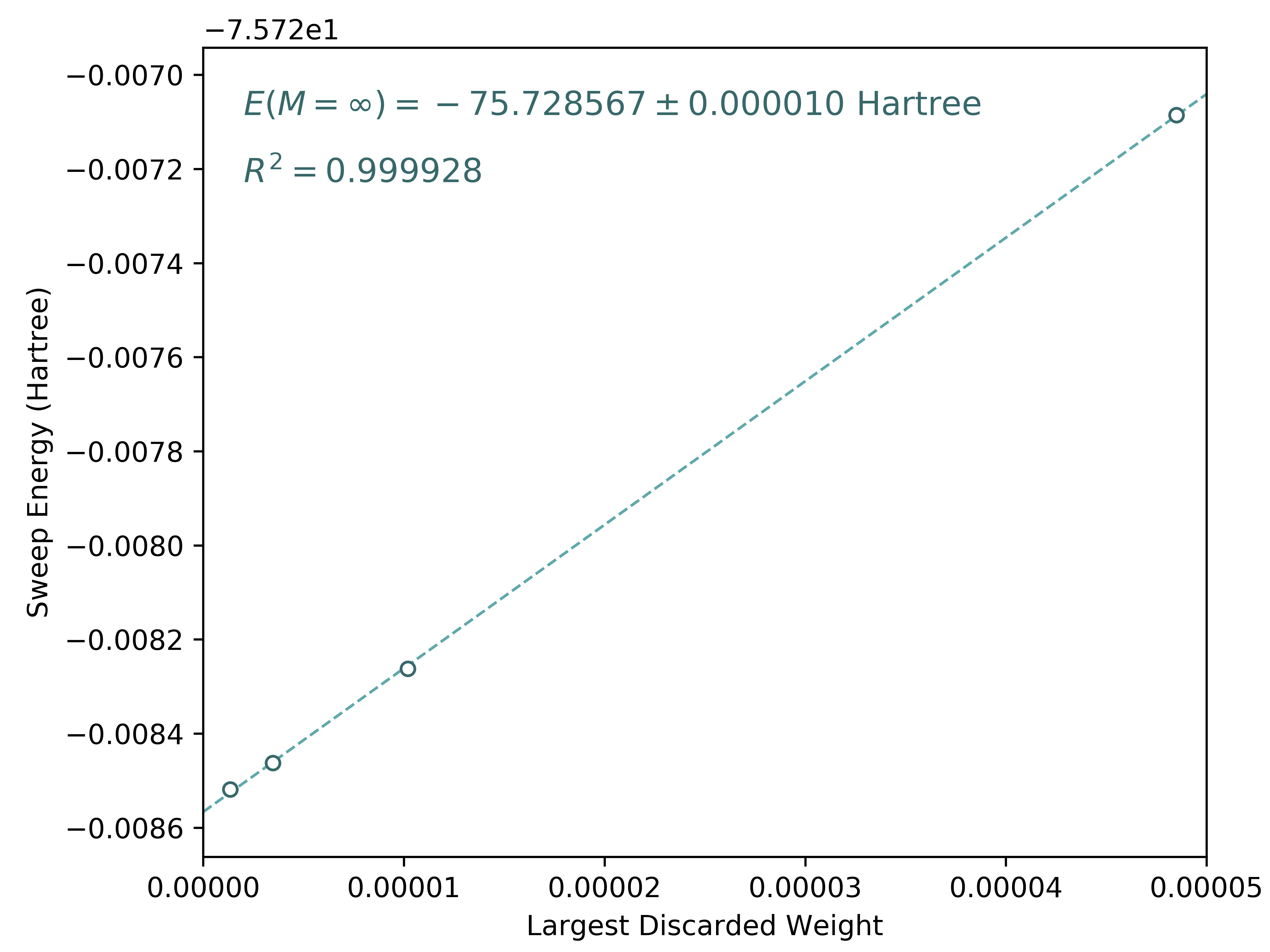
In the above script, we have used the largest discarded weights and associated sweep energies in the last sweep iteration of each bond dimension (\(M = 800, 600, 400, 200\)) to make linear regression. The extrapolated DMRG sweep energy is -75.728567 Hartree.

[1] (1,2,3,4,5,6,7,8,9)

This is an extension implemented only in the block2 code, which is not available in StackBlock.